JPEG

Old fashion, using classical algorithm (basically DCT)

It's lossy even if you set the quality to 100.

And it has a strange name: Joint Photographic Experts Group (JPEG, /ˈdʒeɪpɛɡ/)

1. RGB to YCbCr

YCbCr consists of 3 different channels: Y is the luminance channel containing brightness information, and Cb and Cr are chrominance blue and chrominance red channels containing color information. In this color space, JPEG can make changes to the chrominance channel to change the image’s color information without affecting the brightness information that is located in the luminance channel.

--- JPEG Compression Explained: https://www.baeldung.com/cs/jpeg-compression

2. Downsample chrominance channels

4:2:0 is commonly used.

More details: https://en.wikipedia.org/wiki/Chroma_subsampling

3. Divide into 8x8 blocks

Literal meaning, no need for elaboration.

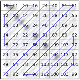
4. Discrete Cosine Transform (DCT)

First, each pixel value for each channel is subtracted by 128 to make the value range from -128 to +127. Then DCT is applied.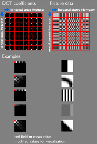

More details of implementation are available here: https://en.wikipedia.org/wiki/JPEG

The DCT result should be like this (for every block):

5. Quantization

The human eye is good at seeing small differences in brightness over a relatively large area, but not so good at distinguishing the exact strength of a high frequency brightness variation. This allows one to greatly reduce the amount of information in the high frequency components. This is done by simply dividing each component in the frequency domain by a constant for that component, and then rounding to the nearest integer. This rounding operation is the only lossy operation in the whole process (other than chroma subsampling) if the DCT computation is performed with sufficiently high precision. As a result of this, it is typically the case that many of the higher frequency components are rounded to zero, and many of the rest become small positive or negative numbers, which take many fewer bits to represent.

--- JPEG - Wikipedia: https://en.wikipedia.org/wiki/JPEG

This is the result:

6. Encoding

Then Huffman coding is used to further reduce the size.

Additional: DCT

The introduction to JPEG introduces Discrete Cosine Transform (DCT), which is a variant of the Discrete Fourier Transform (DFT).

Like the discrete Fourier transform (DFT), a DCT operates on a function at a finite number of discrete data points. The obvious distinction between a DCT and a DFT is that the former uses only cosine functions, while the latter uses both cosines and sines (in the form of complex exponentials). However, this visible difference is merely a consequence of a deeper distinction: a DCT implies different boundary conditions from the DFT or other related transforms.

--- Discrete cosine transform - Wikipedia: https://en.wikipedia.org/wiki/Discrete_cosine_transform

Note the subtle differences at the interfaces between the data and the extensions: in DCT-II and DCT-IV both the end points are replicated in the extensions but not in DCT-I or DCT-III (and a zero point is inserted at the sign reversal extension in DCT-III).

In particular, it is well known that any discontinuities in a function reduce the rate of convergence of the Fourier series, so that more sinusoids are needed to represent the function with a given accuracy. The same principle governs the usefulness of the DFT and other transforms for signal compression; the smoother a function is, the fewer terms in its DFT or DCT are required to represent it accurately, and the more it can be compressed. (Here, we think of the DFT or DCT as approximations for the Fourier series or cosine series of a function, respectively, in order to talk about its "smoothness".) However, the implicit periodicity of the DFT means that discontinuities usually occur at the boundaries: any random segment of a signal is unlikely to have the same value at both the left and right boundaries. (A similar problem arises for the DST, in which the odd left boundary condition implies a discontinuity for any function that does not happen to be zero at that boundary.) In contrast, a DCT where both boundaries are even always yields a continuous extension at the boundaries (although the slope is generally discontinuous). This is why DCTs, and in particular DCTs of types I, II, V, and VI (the types that have two even boundaries) generally perform better for signal compression than DFTs and DSTs. In practice, a type-II DCT is usually preferred for such applications, in part for reasons of computational convenience.

--- Discrete cosine transform - Wikipedia: https://en.wikipedia.org/wiki/Discrete_cosine_transform

There are also other four types of DCT, but they are rarely used.

DCTs of types I–IV treat both boundaries consistently regarding the point of symmetry: they are even/odd around either a data point for both boundaries or halfway between two data points for both boundaries. By contrast, DCTs of types V-VIII imply boundaries that are even/odd around a data point for one boundary and halfway between two data points for the other boundary.

--- Discrete cosine transform - Wikipedia: https://en.wikipedia.org/wiki/Discrete_cosine_transform

PNG

Somewhat modern (using Deflate), and it's lossless!

Portable Network Graphics (PNG, /pɪŋ/)

1. Filter

There is only one filter method in the current PNG specification (denoted method 0), and thus in practice the only choice is which filter type to apply to each line. For this method, the filter predicts the value of each pixel based on the values of previous neighboring pixels, and subtracts the predicted color of the pixel from the actual value, as in DPCM. An image line filtered in this way is often more compressible than the raw image line would be, especially if it is similar to the line above, since the differences from prediction will generally be clustered around 0, rather than spread over all possible image values. This is particularly important in relating separate rows, since DEFLATE has no understanding that an image is a 2D entity, and instead just sees the image data as a stream of bytes.

--- PNG - Wikipedia: https://en.wikipedia.org/wiki/PNG

Now, it’s worth noting that each line may be a little different, which is why PNG allows 1 of 5 different modes to be chosen, per line:

• No filtering
• Difference between X and A
• Difference between X and B
• Difference between X and (A + B)/2 (aka average)
• Paeth predictor (linear function of A, B, C)

--- How PNG Works: https://medium.com/@duhroach/how-png-works-f1174e3cc7b7

The Paeth filter is to choose difference between X and A, B or C, whichever is closest to p = A + B − C.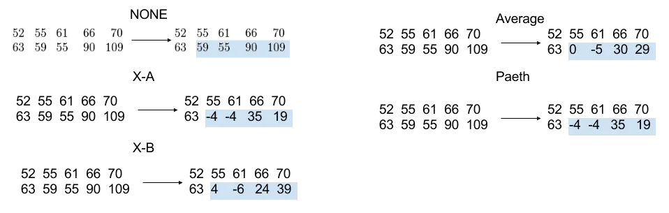

And, it’s important to note that these filters are done, per channel not per-pixel. Meaning that the filter is applied to all the red values of a pixel for a scanline, and then separately for all the blue values for a scanline (although all the colors in a row will use the same filter).

--- How PNG Works: https://medium.com/@duhroach/how-png-works-f1174e3cc7b7

2. Deflate

Deflate (stylized as DEFLATE) is a lossless data compression file format that uses a combination of LZ77 and Huffman coding.

A Deflate stream consists of a series of blocks. Each block is preceded by a 3-bit header:

• First bit: Last-block-in-stream marker:
  • 1: This is the last block in the stream.
  • 0: There are more blocks to process after this one.
• Second and third bits: Encoding method used for this block type:
  • 00: A stored (a.k.a. raw or literal) section, between 0 and 65,535 bytes in length
  • 01: A static Huffman compressed block, using a pre-agreed Huffman tree defined in the RFC
  • 10: A dynamic Huffman compressed block, complete with the Huffman table supplied
  • 11: Reserved—don't use.

The stored block option adds minimal overhead and is used for data that is incompressible.

Most compressible data will end up being encoded using method 10, the dynamic Huffman encoding, which produces an optimized Huffman tree customized for each block of data individually. Instructions to generate the necessary Huffman tree immediately follow the block header. The static Huffman option is used for short messages, where the fixed saving gained by omitting the tree outweighs the percentage compression loss due to using a non-optimal (thus, not technically Huffman) code.

Compression is achieved through two steps:

• The matching and replacement of duplicate strings with pointers.
• Replacing symbols with new, weighted symbols based on the frequency of use.

--- Deflate - Wikipedia: https://en.wikipedia.org/wiki/Deflate

We are all very familiar with Huffman coding, so only duplicate string elimination will be discussed.

Within compressed blocks, if a duplicate series of bytes is spotted (a repeated string), then a back-reference is inserted, linking to the previous location of that identical string instead. An encoded match to an earlier string consists of an 8-bit length (3–258 bytes) and a 15-bit distance (1–32,768 bytes) to the beginning of the duplicate. Relative back-references can be made across any number of blocks, as long as the distance appears within the last 32 KiB of uncompressed data decoded (termed the sliding window).

--- Deflate - Wikipedia: https://en.wikipedia.org/wiki/Deflate